Introduction
The purpose of this article is to describe how to implement an optimized KD tree for raytracing (or other rendering engine) in Rust. The choice of language is arbitrary and should not disturb a non-rustacean (who doesn't code in rust) reader.
The implementation I will use is described in the scientific paper On building fast kd-Trees for Ray Tracing, and on doing that in O(N log N). Since this paper describes well the theoretical part, I will focus on the implementation. However, if you just want to implement a KD tree without diving into the paper formulas, you can keep reading without woring.
Note: There is another acceleration structure called BVH. This one is close to a KD-tree with the difference that it separates shapes instead of space. It is better to use a BVH if you implement it on the GPU or if you want to update the position of the shapes (useful for animation).
This article describes the implementation of several versions of KDTree starting from a naive version to an optimized version. The final and most optimized version is available on github.
The models used for benchmark are from the Stanford Scanning Repository.
General principles
Context
Many rendering engines are based on the physics of light rays (such as raytracer). This method allows to obtain realistic images, but is quite slow. Indeed, it requires throwing a lot of rays and checking if they intersect an object in the scene.
To do this, the easiest way is to check for each shapes (for example triangles) of the scene if it intersects the ray. Even if you have an efficient way to check this intersection, it cannot be viable for a scene with billions of shapes.
The most common solution to this problem is the use of KD tree data structures.
KD what?
Theory
KD tree is a data structure that organize a k-dimensional space. In
our case the k is 3 since we want to organize
the space of our 3D scenes.
KD trees are full binary trees. This means that each internal node contains exactly two children.
They are formed as follows:
- Internal nodes divide the space in half in a selected dimension. They create a sub-space for each child.
- Leaves contain a set of objects that are in their sub-space.
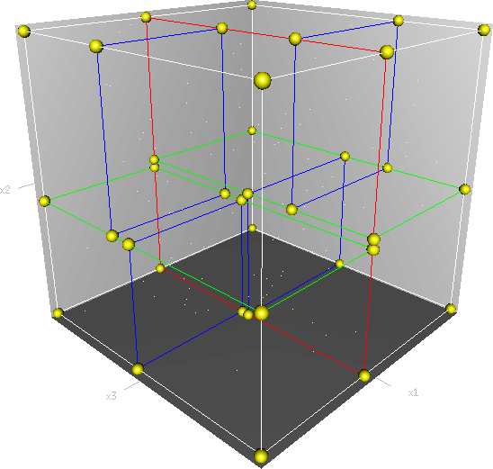
It is important to note that if a shapes (e.g. triangle) is large enough and intersects several cells (subspaces) then this shape will be found in several leaves of our KDTree.
How to build it?
Remember that the goal is to know which shapes intersect a ray without having to check each of them. The idea is to provide a reduced list of shape candidates that could intersect a ray. So the quality of our KD tree depends on three things:
- The number of candidates returned by our KD tree.
- The time taken by the KD tree to generate the list.
- The time taken to create the KD tree. This point can be considered less important since the tree is built only once.
During our construction, we will have to check if the shape intersect a sub-space or not to be able to arrange them in the right node of the tree. To do so sub-space and shapes will be described by a 3D AABB (Axis-aligned bounding boxes).
An AABB is convenient and optimized to check if two entities overlap. It is also simple to check if a ray intersects an AABB.
So, to build a KD tree, we must recursively divide a space and classify which shapes overlap the new subspaces. For an optimal KDTree, we must divide the space optimally and stop recursion optimally.
Naive implementation
This version will serve as a proof of concept. And yet, it will significantly reduce the intersection search algorithm runtime.
Needed structure
Bounding Box
First of all, we have to define our AABB since that's what we're going to manipulate. We also implement some useful methods.
AABB::newwill create a new AABB from two points.AABB::emptywill create an empty AABB that can't intersect anything.AABB::mergewill merge two AABBs into one. Behaves like a union.AABB::intersect_boxwill check if our AABB overlap with another AABB.
use cgmath::*;

// Define a point3 and a vector3 type to make the code more readable.
type Point3 = cgmath::Vector3<f32>;
type Vector3 = cgmath::Vector3<f32>;

/// Axis-aligned bounding box is defined by two positions.
#[derive(Clone, Debug)]
pub struct AABB {
    /// Minimum position
    pub min: Point3,
    /// Maximum position
    pub max: Point3,
}

impl AABB {
    /// Create an new AABB from two points.
    pub fn new(min: Point3, max: Point3) -> Self {
        Self { min, max }
    }

    /// Create an empty AABB.
    pub fn empty() -> Self {
        Self::new(
            Point3::new(f32::INFINITY, f32::INFINITY, f32::INFINITY),
            Point3::new(f32::NEG_INFINITY, f32::NEG_INFINITY, f32::NEG_INFINITY),
        )
    }

    /// Check the intersection with another box.
    pub fn intersect_box(&self, other: &AABB) -> bool {
       (self.0.x < other.1.x && self.1.x > other.0.x)
           && (self.0.y < other.1.y && self.1.y > other.0.y)
           && (self.0.z < other.1.z && self.1.z > other.0.z)
    }

    /// Merge another AABB into this one.
    pub fn merge(&mut self, other: &Self) {
        self.min = Point3::new(
            self.min.x.min(other.min.x),
            self.min.y.min(other.min.y),
            self.min.z.min(other.min.z),
        );
        self.max = Point3::new(
            self.max.x.max(other.max.x),
            self.max.y.max(other.max.y),
            self.max.z.max(other.max.z),
        );
    }
}

impl Default for AABB {
    fn default() -> Self {
        Self::empty()
    }
}
We need a function to check if a ray intersect an AABB
(Ray::intersect). It's extremely important to optimize this
function. We will use an internal representation of a ray with
precompute values to speed up the intersection check.
Check scratchapixel for more info about the math.
/// A 3D ray
pub struct Ray {
    /// The origin of the ray
    origin: Vector3,
    /// The inverse of the direction of the ray (1 / direction)
    inv_direction: Vector3,
    /// The sign of the direction of the ray (0 if negative, 1 if positive)
    sign: [bool; 3],
}

impl Ray {
    pub fn new(origin: &Vector3, direction: &Vector3) -> Self {
        let inv_direction = Vector3::new(1. / direction.x, 1. / direction.y, 1. / direction.z);
        let sign = [direction.x < 0., direction.y < 0., direction.z < 0.];

        Self {
            origin: *origin,
            inv_direction,
            sign,
        }
    }

    fn get_aabb_sign(aabb: &AABB, sign: bool) -> Point3 {
        if sign {
            aabb.max
        } else {
            aabb.min
        }
    }

    pub fn intersect(&self, aabb: &AABB) -> bool {
        let mut ray_min =
            (Self::get_aabb_sign(aabb, self.sign[0]).x - self.origin.x) * self.inv_direction.x;
        let mut ray_max =
            (Self::get_aabb_sign(aabb, !self.sign[0]).x - self.origin.x) * self.inv_direction.x;

        let y_min =
            (Self::get_aabb_sign(aabb, self.sign[1]).y - self.origin.y) * self.inv_direction.y;
        let y_max =
            (Self::get_aabb_sign(aabb, !self.sign[1]).y - self.origin.y) * self.inv_direction.y;

        if (ray_min > y_max) || (y_min > ray_max) {
            return false;
        }

        // Using the following solution significantly decreases the performance
        // ray_min = ray_min.max(y_min);
        if y_min > ray_min {
            ray_min = y_min;
        }

        // Using the following solution significantly decreases the performance
        // ray_max = ray_max.min(y_max);
        if y_max < ray_max {
            ray_max = y_max;
        }

        let z_min =
            (Self::get_aabb_sign(aabb, self.sign[2]).z - self.origin.z) * self.inv_direction.z;
        let z_max =
            (Self::get_aabb_sign(aabb, !self.sign[2]).z - self.origin.z) * self.inv_direction.z;

        if (ray_min > z_max) || (z_min > ray_max) {
            return false;
        }

        // Using the following solution significantly decreases the performance
        // ray_max = ray_max.min(y_max);
        if z_max < ray_max {
            ray_max = z_max;
        }

        ray_max > 0.0
    }
}
Finally, we need a trait that our shapes will have to implement. So we can retrieve an AABB for the given shapes.
pub trait Bounded {
    fn bound(&self) -> AABB;
}
KD Tree Structs
It's time to create the structure of our KDTree. A
KDTree is above all a binary tree. The most optimized way in memory and
in browsing is a list where each element represents a node. If it is an
internal node then it contains the index of its left and right child,
otherwise it contains only the leaf information.

In addition of a list of nodes we need a global space
AABB that contains all the shapes of our tree. It can be
interesting to know the maximum depth of our tree. It can
be useful to make some optimizations during its traversal.
/// The KD-tree data structure.
#[derive(Clone, Debug)]
pub struct KDTree {
    tree: Vec<KDTreeNode>,
    space: AABB,
    depth: usize,
}
Now we can now define our KDTreeNode. In rust
enum are perfect for this kind of object. It allows us to
define two state:
Leaf: Represents a leaf of our tree.Node: Represents an internal node of our tree.
#[derive(Clone, Debug)]
pub enum KDTreeNode {
    Leaf {
        shapes: Vec<usize>,
    },
    Node {
        l_child: usize,
        l_space: AABB,
        r_child: usize,
        r_space: AABB,
    },
}
The implementation of this structure is really important.
- Shapes are stored in a
Vec. We useusizethat represent a unique id for each shape. This id is the index of the shape in the collection of shapes given as input of our construction.
The first element of our tree is the root of the tree. The second element will be the left child of the root and so on.
Plane
Let's create a structure that represents a split in a space. Since our space is in 3D a plane is perfect to represents this seperation. We will add some utility functions.
/// 3D dimensions enum.
#[derive(Clone, Copy, Debug, PartialEq, Eq, Hash, Enum)]
pub enum Dimension {
    X,
    Y,
    Z,
}

// This is implementation details.
// EnumMap behaves like HashMap but are implemented as an array since the key is a variant.
impl Dimension {
    pub fn get_map<T: Clone>(value: T) -> EnumMap<Dimension, T> {
        enum_map! {
            Dimension::X => value.clone(),
            Dimension::Y => value.clone(),
            Dimension::Z => value.clone()
        }
    }
}

/// 3D plane.
#[derive(Clone, Debug)]
pub struct Plane {
    pub dimension: Dimension,
    pub pos: f32,
}

impl Plane {
    /// Create a new plane.
    pub fn new(dimension: Dimension, pos: f32) -> Self {
        Plane { dimension, pos }
    }

    /// Create a new plane on the X axis.
    pub fn new_x(pos: f32) -> Self {
        Plane::new(Dimension::X, pos)
    }

    /// Create a new plane on the Y axis.
    pub fn new_y(pos: f32) -> Self {
        Plane::new(Dimension::Y, pos)
    }

    /// Create a new plane on the Z axis.
    pub fn new_z(pos: f32) -> Self {
        Plane::new(Dimension::Z, pos)
    }
}
Build KDTree
KDTree
Let's first implement the function that build a KDTree.
To do so we need a list of shapes. The function will compute the initial
space of the KDTree and create the root node.
impl KDTree {
    /// This function is used to build a new KDTree. You need to provide a
    /// `Vec` of shapes that implement `Bounded` trait.
    pub fn build<S: Bounded>(mut shapes: &Vec<S>) -> Self {
        let mut space = Default::default();
        // Contains all the items (id and bounding box)
        let mut items = Vec::new();
        // Enumerate the shapes to get a tuple (id, value)
        for (index, shape) in shapes.iter().enumerate() {
            // Create bounding box from the shape
            let bb = shape.bound();

            // Update space with the bounding box of the item
            space.merge(&bb);

            // Add the item to the list
            items.push((index, bb));
        }

        // Create a tree with a maximum depth of 10. It will fill inplace the tree.
        let mut tree = vec![];
        let depth = build_tree(&space, items, 10, &mut tree);
        KDTree { space, tree, depth }
    }
}
Note that the maximum depth will allow us to create a stopping criterion easily. The value was chosen arbitrarily.
Tree
Let's implement the function that will actually build the tree.
/// Naive implementation to build a KDTree. Returns the depth of the tree.
pub fn build_tree(
    space: &AABB,
    items: Vec<(usize, AABB)>,
    max_depth: usize, tree:
    &mut Vec<KDTreeNode>
) -> usize {
    // Heuristic to terminate the recursion
    if items.len() <= 15 || max_depth == 0 {
        // Create a push the leaf
        let shapes = items.into_iter().map(|(id, _)| id).collect();
        tree.push(KDTreeNode::Leaf { shapes });
        return 1;
    }

    // Find a plane to partition the space
    let plane = Self::partition(&space, max_depth);

    // Compute the new spaces divided by `plane`
    let (left_space, right_space) = split_space(&space, &plane);

    // Compute which items are part of the left and right space
    let (left_items, right_items) =
        classify(&items, &left_space, &right_space);

    let node_index = tree.len();
    tree.push(KDTreeNode::Node {
        l_child: node_index + 1,
        l_space: left_space.clone(),
        r_child: 0, // Filled later
        r_space: right_space.clone(),
    });

    // Add left child
    let depth_left = build_tree(&left_space, left_items, max_depth - 1, tree);

    let r_child_index = tree.len();
    tree[node_index].set_r_child_index(r_child_index);

    // Add right
    let depth_right = build_tree(&right_space, right_items, max_depth - 1, tree);

    // Return the depth of the tree
    1 + depth_left.max(depth_right)
}
There is a lot going on here. This contains the basic algorithm to build our KDTree. Note that an arbitrary heuristic is used. The effectiveness of this heuristic depends mainly on the scene itself. We can greatly improve it by using more parameters but we will talk about it later.
We still need to implement the functions classify,
split_space and partition. This last function
is probably the most important since, depending on where we split our
space, the KDTree will be more or less efficient. Once again we're going
to take the most simple solution for now. We will use the spatial
median splitting technique. At each depth of the tree,
the axis on which the division is made will be changed.
fn classify(items: &Vec<(usize, AABB)>, left_space: &AABB, right_space: &AABB)
  -> (Vec<(usize, AABB)>, Vec<(usize, AABB)>) {
    (
        // All items that overlap with the left space is taken
        items
            .iter()
            .filter(|item| left_space.intersect_box(&item.bb))
            .cloned()
            .collect(),
        // All items that overlap with the right space is taken
        items
            .iter()
            .filter(|item| right_space.intersect_box(&item.bb))
            .cloned()
            .collect(),
    )
}

fn split_space(space: &AABB, plane: &Plane) -> (AABB, AABB) {
    let mut left = space.clone();
    let mut right = space.clone();
    let pos = splitting_plane.pos;
    match splitting_plane.dimension {
        Dimension::X => {
            right.min.x = pos.clamp(space.min.x, space.max.x);
            left.max.x = pos.clamp(space.min.x, space.max.x);
        }
        Dimension::Y => {
            right.min.y = pos.clamp(space.min.y, space.max.y);
            left.max.y = pos.clamp(space.min.y, space.max.y);
        }
        Dimension::Z => {
            right.min.z = pos.clamp(space.min.z, space.max.z);
            left.max.z = pos.clamp(space.min.z, space.max.z);
        }
    }
    (left, right)
}

fn partition(space: &AABB, max_depth: usize) -> Plane {
    match max_depth % 3 {
        0 => Plane::new_x((space.min.x + space.max.x) / 2.),
        1 => Plane::new_y((space.min.y + space.max.y) / 2.),
        _ => Plane::new_z((space.min.z + space.max.z) / 2.),
    }
}
You may have noticed that the split_space function clips
the plane to the space. This is perfectly useless for the
naive version. The median plane will never be outside the
space. However later versions might call the function with
a plane that is not contained in space.
Intersect KD Tree
Now that our KDTree is built, we are able to compute our reduced list of shapes that can intersect a ray.
impl KDTree {

    /// This function takes a ray and return a reduced list of shapes that
    /// can be intersected by the ray.
    pub fn intersect(&self, ray_origin: &Vector3, ray_direction: &Vector3) -> Vec<usize> {
        let ray = Ray::new(ray_origin, ray_direction);
        let mut result = vec![];
        let mut stack = vec![0];
        // Reserve enough space for the stack to avoid reallocation.
        stack.reserve_exact(self.depth);
        while !stack.is_empty() {
            let node = &self.tree[stack.pop().unwrap()];
            match node {
                KDTreeNode::Leaf { shapes } => result.extend(shapes),
                KDTreeNode::Node { l_child, l_space, r_child, r_space } => {
                    if ray.intersect(r_space) {
                        stack.push(*r_child)
                    }
                    if ray.intersect(l_space) {
                        stack.push(*l_child)
                    }
                }
            }
        }
        // Dedup duplicated shapes
        result.sort();
        result.dedup();
        result
    }
}
The KDTree::intersect is responsible to walk through the
KDTree and fill all the candidates shapes in a vector. Then we remove
duplicate in this vector; I tried multiple implementation here (set,
keep a sorted vec, ...). The most efficient one is to sort and dedup
items at the end.
We are done with our naive implementation. It is obvious that a lot could be done to improve the generated tree and we will explore this in the next part. Still, this implementation brings a huge improvement to our rendering engine.
Surface Area Heuristic (SAH)
Theory
The SAH method provides both the ability to know which cutting plane is the best and whether it is worth dividing the space (create a node) or not (create a sheet). To do this, we need to calculate the "cost" of a leaf and the internal nodes for each possible splitting plane.
Before explaining the method, we need to make a few assumptions:
- \(K_I\): The cost for shapes Intersection.
- \(K_T\): The cost for a Traversal step of the tree.
We can now calculate the cost of an intersection in our kd-tree. Let's say that, for a given ray and kd-tree, the intersection function returns 13 shapes and had to pass through 8 nodes of the tree.
\(C_{intersection} = 13 \times K_I + 8 \times K_T\).
It is fairly easy to calculate the cost of a leaf. It is simply the number of shapes contained in the leaf \(|T|\) multiplied by \(K_I\).
\(C_{leaf} = |T| \times K_I\)
It is somewhat more difficult to calculate the cost of an internal node given a splitting plane. First we need to define more terms:
- \(p\): The splitting plane candidate.
- \(V\): The space of the whole node.
- \(|V_L|\) and \(|V_R|\): The left and right space splitted by \(p\).
- \(|T_L|\) and \(|T_R|\): The number of shapes that overlap the left and right volumes seperated by \(p\).
- \(SA(space)\): The function that calculate the surface area of a given space. This function is quite simple knowing the spaces are AABB, it's simply the sum of the surfaces of each side of the box.
For a box of length \(V_{length}\), width \(V_{width}\) and height \(V_{height}\), the surface area is:
\(SA(V) = 2 \times (V_{length} \times V_{width} + V_{length} \times V_{height} + V_{width} \times V_{height})\)
The cost of an internal node is given by the following formula.
\(C_{node}(p) = K_T + K_I \Big (|T_L| \times \frac{SA(V_L)}{SA(V)} + |T_R| \times \frac{SA(V_R)}{SA(V)} \Big)\)
This formula may seem magical, but it is simply the cost of one traversal step (\(K_T\)), plus the expected cost of intersecting the two children. The expected cost of intersecting a child is calculated by multiplying the number of shapes in the child and the ratio of the surface taken by the child's space.
Some shortcuts were made in the explanation of the formulas for more details take a look at the scientific reference paper.
One last thing, we can add a bonus for cutting space with no shapes is in one of the children. The paper suggest to reduced the computed cost by \(80\%\).
How to use SAH
Sah gives us a way to compare splitting planes and select the best one. Once we have it, Sah lets us know if it's worth cutting or if a leaf is preferable.
Basically what will change in our code is the partition function and the termination function.
To divide our space, we are going to take all the possible splitting planes in the 3 dimensions (called perfect splits). Then we will calculate the cost of the partition and take the smallest one.
We need to define K_T and K_I in our implementation. For this the paper advice to use:
- \(K_T=15\)
- \(K_I=20\)
Implementation of needed functions
These are the functions that use the above formulas to calculate the cost of a split.
impl AABB {
    /// Compute AABB surface
    pub fn surface(&self) -> f32 {
        let dx = self.max.x - self.min.x;
        let dy = self.max.y - self.min.y;
        let dz = self.max.z - self.min.z;
        2.0 * (dx * dy + dx * dz + dy * dz)
    }
}

impl Plane {
    /// Check if the plane is cutting the given space.
    pub fn is_cutting(&self, space: &AABB) -> bool {
        match self.dimension {
            Dimension::X => self.pos > space.min.x && self.pos < space.max.x,
            Dimension::Y => self.pos > space.min.y && self.pos < space.max.y,
            Dimension::Z => self.pos > space.min.z && self.pos < space.max.z,
        }
    }
}

static K_T: f32 = 15.;
static K_I: f32 = 20.;
/// Bonus (between `0.` and `1.`) for cutting an empty space:
/// * `1.` means that cutting an empty space is in any case better than cutting a full space.
/// * `0.` means that cutting an empty space isn't better than cutting a full space.
static EMPTY_CUT_BONUS: f32 = 0.2;

/// Surface Area Heuristic (SAH)
fn cost(plane: &Plane, space: &AABB, n_left: usize, n_right: usize) -> f32 {
    // If the plane doesn't cut the space, return max cost
    if !plane.is_cutting(space) {
        return f32::INFINITY;
    }

    // Compute the surface area of the whole space
    let surface_space = space.surface();

    // Split space
    let (space_left, space_right) = split_space(space, plane);

    // Compute the surface area of both subspace
    let surface_left = space_left.surface();
    let surface_right = space_right.surface();

    // Compute raw cost
    let cost = K_T + K_I
            * (n_left as f32 * surface_left / surface_space
                + n_right as f32 * surface_right / surface_space);

    // Decrease cost if it cuts empty space
    if n_left == 0 || n_right == 0 {
        cost * (1. - EMPTY_CUT_BONUS)
    } else {
        cost
    }
}
The cost formula is slightly different from the one presented above. If the splitting plane doesn't cut the space, we return \(\infty\).
Generate candidates
We are able to evaluate the cost of a split. However, there remains a problem, in a given space there are an infinite number of planes of partition. It is therefore necessary to choose an arbitrary number of planes that we will compare with each other and select the one with the lowest cost. These planes will be called candidates.
We can observe that in a given dimension two different planes that separate the elements in the same way will have a very close cost. This being said we can choose as candidates the planes formed by the sides of the bounding boxes of each shapes.

Given the bounding box of a shape and a dimension we need to be able to generate such splitting candidates.
pub fn candidates(space: &AABB, dim: Dimension) -> Vec<Plane> {
    match dim {
        Dimension::X => vec![Plane::new_x(space.bb.min.x), Plane::new_x(space.bb.max.x)],
        Dimension::Y => vec![Plane::new_y(space.bb.min.y), Plane::new_y(space.bb.max.y)],
        Dimension::Z => vec![Plane::new_z(space.bb.min.z), Plane::new_z(space.bb.max.z)],
    }
}
Build tree in \(O(N^2)\)
We can update the partition and build_tree
functions to get rid of our heuristics and use the sah instead (no more
max_depth). This modification will greatly increase the
construction time of the KDTree. We will ignore this for now.
pub fn build_tree(
    space: &AABB,
    items: Vec<(usize, AABB)>,
    &mut Vec<KDTreeNode>
) -> usize {
    let (cost, plane) = partition(&space, &items);

    // Check that the cost of the splitting is not higher than the cost of
    // the leaf.
    if cost > K_I * items.len() as f32 {
        // Create a push the leaf
        let shapes = items.into_iter().map(|(id, _)| id).collect();
        tree.push(KDTreeNode::Leaf { shapes });
        return 1;
    }

    // Compute the new spaces divided by `plane`
    let (left_space, right_space) = split_space(&space, &plane);

    // Compute which items are part of the left and right space
    let (left_items, right_items) =
        classify(&items, &left_space, &right_space);

    let node_index = tree.len();
    tree.push(KDTreeNode::Node {
        l_child: node_index + 1,
        l_space: left_space.clone(),
        r_child: 0, // Filled later
        r_space: right_space.clone(),
    });

    // Add left child
    let depth_left = build_tree(&left_space, left_items, max_depth - 1, tree);

    let r_child_index = tree.len();
    tree[node_index].set_r_child_index(r_child_index);

    // Add right
    let depth_right = build_tree(&right_space, right_items, max_depth - 1, tree);

    // Return the depth of the tree
    1 + depth_left.max(depth_right)
}

/// Takes the items and space of a node and return the best splitting plane
/// and his cost
fn partition(space: &AABB, items: &Vec<(usize, AABB)>) -> (f32, Plane) {
    let (mut best_cost, mut best_plane) = (f32::INFINITY, Plane::new_x(0.));
    // For all the dimension
    for dim in [Dimension::X, Dimension::Y, Dimension::Z] {
        for (_, shape_space) in items {
            for plane in candidates(shape_space, dim) {
                // Compute the new spaces divided by `plane`
                let (left_space, right_space) = split_space(&space, &plane);

                // Compute which items are part of the left and right space
                let (left_items, right_items) = classify(&items, &left_space, &right_space);

                // Compute the cost of the current plane
                let cost = cost(&plane, space, left_items.len(), right_items.len());

                // If better update the best values
                if cost < best_cost {
                    best_cost = cost;
                    best_plane = plane.clone();
                }
            }
        }
    }
    (best_cost, best_plane)
}
For each candidate, we call classify
function that performs an iteration on all items. This is why this
partition implementation is in \(O(N^2)\). As you can check in the Benchmark section, this implementation is not
viable.
Build tree in \(O(N \log^2{N})\)
Let's now optimize the construction time of our KDTree. We noticed
that the element that makes our construction slow is the usage of the
function classify.
The reason for calling this function is to find out the number of items to the left and right of a splitting candidate. To solve this problem we will use an incremental sweep algorithm.
This algorithm needs to know if a splitting candidate is to the left or to the right of its associated shapes.
In a given dimension, two counters are established:
- The number of shapes to the left of the candidate.
- The number of shapes to the right of the candidate.
These are the necessary information for the cost
function. The algorithm will then sweep the candidates in the order of
their position and depending on whether they are to the left or to the
right of the shape it will update its counters.
Here is a diagram to illustrate the steps of the algorithm.

| Candidates | Side | Left count | Right count |
|---|---|---|---|
| Initialization | N/A | 0 | 3 |
| 1 | Left | 0 + 1 = 1 | 3 |
| 2 | Left | 1 + 1 = 2 | 3 |
| 3 | Right | 2 | 3 - 1 = 2 |
| 4 | Left | 2 + 1 = 3 | 2 |
| 5 | Right | 3 | 2 - 1 = 1 |
| 6 | Right | 3 | 1 - 1 = 0 |
You may have noticed that the left counter has not exactly the right value. There is an offset when the candidate is left. You will have to update the counter value after calling the cost function.
The same kind of function can be used to find the items belonging to the left and right subspace. But for this purpose the candidates must keep the id on their associated shape.
Candidate
A Candidate structure is needed to aggregate the
separator planes, their side (left/right) and the shape id.
We will also add some utility functions to create a new candidate,
and retrieve information such as their dimension, value, and side. We
implement a function to generate these candidates similar to the
previous function candidates.
/// Candidates is a list of Candidate
pub type Candidates = Vec<Candidate>;

#[derive(Debug, Clone)]
pub struct Candidate {
    pub plane: Plane,
    pub is_left: bool,
    pub shape: usize,
    pub space: AABB,
}

impl Candidate {
    fn new(plane: Plane, is_left: bool, index: usize, space: AABB) -> Self {
        Candidate {
            plane,
            is_left,
            shape: index,
            space,
        }
    }

    /// Return candidates (splits candidates).
    pub fn gen_candidates(shape: usize, bb: &AABB, dim: Dimension) -> Candidates {
        match dim {
            Dimension::X => vec![
                Candidate::new(Plane::new_x(bb.min.x), true, shape, bb.clone()),
                Candidate::new(Plane::new_x(bb.max.x), false, shape, bb.clone()),
            ],
            Dimension::Y => vec![
                Candidate::new(Plane::new_y(bb.min.y), true, shape, bb.clone()),
                Candidate::new(Plane::new_y(bb.max.y), false, shape, bb.clone()),
            ],
            Dimension::Z => vec![
                Candidate::new(Plane::new_z(bb.min.z), true, shape, bb.clone()),
                Candidate::new(Plane::new_z(bb.max.z), false, shape, bb.clone()),
            ],
        }
    }

    pub fn dimension(&self) -> Dimension {
        self.plane.dimension
    }

    pub fn position(&self) -> f32 {
        self.plane.pos
    }

    pub fn is_left(&self) -> bool {
        self.is_left
    }

    pub fn is_right(&self) -> bool {
        !self.is_left
    }
}Important: The function gen_candidates
returns first the left candidate and then the right one. This detail is
important. If the bounding box of the item is flat (so that its
candidates have the same value), the left candidate must still appear
first during the sweep.
We also need to be able to sort the candidates. For this we implement
the trait Ord and Eq.
impl Ord for Candidate {
    fn cmp(&self, other: &Self) -> Ordering {
        if self.position() < other.position() {
            Ordering::Less
        } else {
            Ordering::Greater
        }
    }
}
impl PartialOrd for Candidate {
    fn partial_cmp(&self, other: &Self) -> Option<Ordering> {
        Some(self.cmp(other))
    }
}

impl PartialEq for Candidate {
    fn eq(&self, other: &Self) -> bool {
        self.position() == other.position() && self.dimension() == other.dimension()
    }
}

impl Eq for Candidate {}
Partition and Classify
The partition function will have a lot of modification
first instead of returning a Plane we will return the
sorted list of candidates and the index of the best splitting candidate.
Doing so will allow us to use an optimized classify function.
/// Compute the best splitting candidate
/// Return:
/// * Cost of the split
/// * The list of candidates (in the best dimension found)
/// * Index of the best candidate
fn partition(items: &Vec<(usize, AABB)>, space: &AABB) -> (f32, Candidates, usize) {
    let mut best_cost = f32::INFINITY;
    let mut best_candidate_index = 0;
    let mut best_candidates = vec![];

    // For all the dimension
    for dim in [Dimension::X, Dimension::Y, Dimension::Z] {
        // Generate candidates
        let mut candidates = vec![];
        for (shape_index, shape_aabb) in items {
            let mut c = Candidate::gen_candidates(shape_index, shape_aabb, dim);
            candidates.append(&mut c);
        }

        // Sort candidates
        candidates.sort();

        // Initialize counters
        let mut n_r = items.len();
        let mut n_l = 0;

        // Used to update best_candidates list
        let mut best_dim = false;

        // Find best candidate
        for (i, candidate) in candidates.iter().enumerate() {
            if candidate.is_right() {
                n_r -= 1;
            }

            // Compute the cost of the current plane
            let cost = cost(&candidate.plane, space, n_l, n_r);

            // If better update the best values
            if cost < best_cost {
                best_cost = cost;
                best_candidate_index = i;
                best_dim = true;
            }

            if candidate.is_left() {
                n_l += 1;
            }
        }

        // If a better candidate was found then keep the candidate list
        if best_dim {
            best_candidates = candidates;
        }
    }
    (best_cost, best_candidates, best_candidate_index)
}
It is important to know that sorting in Rust is stable, i.e. in our
case that two candidates having the same plan will keep their order.
This is important to correctly handle the case of the flat bounding box.
If you use a non-stable sort you can slightly modify the candidate
comparison function to take into account the is_left
field.
The classify function is quite simple to implement.
fn classify(candidates: &Candidates, best_index: usize)
  -> (Vec<(usize, AABB)>, Vec<(usize, AABB)>) {
    let mut left_items = Vec::with_capacity(candidates.len() / 2);
    let mut right_items = Vec::with_capacity(candidates.len() / 2);

    for i in 0..best_index {
        if candidates[i].is_left() {
            left_items.push((candidates[i].shape, candidates[i].space));
        }
    }
    for i in (1 + best_index)..candidates.len() {
        if candidates[i].is_right() {
            right_items.push((candidates[i].shape, candidates[i].space));
        }
    }
    (left_items, right_items)
}
Finally we must adapt the function build_tree.
pub fn build_tree(
    space: &AABB,
    items: Vec<(usize, AABB)>,
    &mut Vec<KDTreeNode>
) -> usize {
    let (cost, candidates, best_index) = partition(&space, &items);

    // Check that the cost of the splitting is not higher than the cost of
    // the leaf.
    if cost > K_I * items.len() as f32 {
        // Create a push the leaf
        let shapes = items.into_iter().map(|(id, _)| id).collect();
        tree.push(KDTreeNode::Leaf { shapes });
        return 1;
    }

    // Compute the new spaces divided by `plane`
    let (left_space, right_space) = split_space(&space, &candidates[best_idnex].plane);

    // Compute which items are part of the left and right space
    let (left_items, right_items) = classify(&candidates, best_index);

    // The rest of the function is the same as before
    // [...]
}
We now have a correct implementation of KDTree. However we can still speed up the tree construction to be optimal. We will see how in the next part.
Build tree in \(O(N \log{N})\)
This slows down our tree construction and the sorting of candidates. The idea to optimize is to do one sort at the very beginning.
To do this we have to solve two problems:
- Take the sorting out of the inner loop of the
partitionfunction. - Classify the candidates keeping them sorted.
The first problem can be fixed easily if we take as an argument a sorted list of candidates (from all dimension) we can easily find the best candidate. We just need more counters and be careful of candidates dimension.
We can modify our partition function:
/// Compute the best splitting candidate
/// Return:
/// * Cost of the split
/// * Index of the best candidate
/// * Number of items in the left partition
/// * Number of items in the right partition
fn partition(
    n: usize,
    space: &AABB,
    candidates: &Candidates,
) -> (f32, usize, usize, usize) {
    let mut best_cost = f32::INFINITY;
    let mut best_candidate_index = 0;

    // Variables to keep count the number of items in both subspace for each dimension
    let mut n_l = Dimension::get_map(0);
    let mut n_r = Dimension::get_map(n);

    // Keep n_l and n_r for the best splitting candidate
    let mut best_n_l = 0;
    let mut best_n_r = n;

    // Find best candidate
    for (i, candidate) in candidates.iter().enumerate() {
        let dim = candidate.dimension();

        // If the right candidate removes it from the right subspace
        if candidate.is_right() {
            n_r[dim] -= 1;
        }

        // Compute the cost of the split and update the best split
        let cost = cost(&candidate.plane, space, n_l[dim], n_r[dim]);
        if cost < best_cost {
            best_cost = cost;
            best_candidate_index = i;
            best_n_l = n_l[dim];
            best_n_r = n_r[dim];
        }

        // If the left candidate add it from the left subspace
        if candidate.is_left() {
            n_l[dim] += 1;
        }
    }
    (best_cost, best_candidate_index, best_n_l, best_n_r)
}
Now we need to split our candidate list given a splitting candidate. Not forgetting to keep our new list sorted. We can do that in two steps:
- Determining which items is in the left/right/both subspace.
- Iterate on candidates adding them to the left/right list of candidates.
To mark items as on left/right/both subspace we can use a new
enum Side and items id field.
/// Useful to classify candidates
#[derive(Debug, Clone, Copy)]
pub enum Side { Left, Right, Both }
Instead of instantiating a list of Side each time we
call the classify function. We can create this list once at the
beginning and pass it through the recursive calls of our tree.
Let's implement our new classify function:
fn classify(
    candidates: Candidates,
    best_index: usize,
    sides: &mut [Side],
) -> (Candidates, Candidates) {
    // Step 1: Udate sides to classify items
    classify_items(&candidates, best_index, sides);

    // Step 2: Splicing candidates left and right subspace
    splicing_candidates(candidates, sides)
}

/// Step 1 of classify.
/// Given a candidate list and a splitting candidate identify wich items are part of the
/// left, right and both subspaces.
fn classify_items(candidates: &Candidates, best_index: usize, sides: &mut [Side]) {
    let best_dimension = candidates[best_index].dimension();
    for i in 0..(best_index + 1) {
        if candidates[i].dimension() == best_dimension {
            if candidates[i].is_right() {
                sides[candidates[i].shape] = Side::Left;
            } else {
                sides[candidates[i].shape] = Side::Both;
            }
        }
    }
    for i in best_index..candidates.len() {
        if candidates[i].dimension() == best_dimension && candidates[i].is_left() {
            sides[candidates[i].shape] = Side::Right;
        }
    }
}

// Step 2: Splicing candidates left and right subspace given items sides
fn splicing_candidates(mut candidates: Candidates, sides: &[Side]) -> (Candidates, Candidates) {
    let mut left_candidates = Candidates::with_capacity(candidates.len() / 2);
    let mut right_candidates = Candidates::with_capacity(candidates.len() / 2);

    for e in candidates.drain(..) {
        match sides[e.shape] {
            Side::Left => left_candidates.push(e),
            Side::Right => right_candidates.push(e),
            Side::Both => {
                right_candidates.push(e.clone());
                left_candidates.push(e);
            }
        }
    }
    (left_candidates, right_candidates)
}
Let's adapt the function build_tree.
/// Build a KDTree from a list of candidates and return the depth of the tree.
pub fn build_tree(
    space: &AABB,
    candidates: Candidates,
    nb_shapes: usize,
    sides: &mut [Side],
    tree: &mut Vec<KDTreeNode>,
) -> usize {
    let (cost, best_index, n_l, n_r) = partition(nb_shapes, space, &candidates);

    // Check that the cost of the splitting is not higher than the cost of the leaf.
    if cost > K_I * nb_shapes as f32 {
        // Create indices values vector
        let shapes = candidates
            .iter()
            .filter(|e| e.is_left() && e.dimension() == Dimension::X)
            .map(|e| e.shape)
            .collect();
        tree.push(KDTreeNode::Leaf { shapes });
        return 1;
    }

    // Compute the new spaces divided by `plane`
    let (left_space, right_space) = split_space(space, &candidates[best_index].plane);

    // Compute which candidates are part of the left and right space
    let (left_candidates, right_candidates) = classify(candidates, best_index, sides);

    // Add current node
    let node_index = tree.len();
    tree.push(KDTreeNode::Node {
        l_child: node_index + 1,
        l_space: left_space.clone(),
        r_child: 0, // Filled later
        r_space: right_space.clone(),
    });

    // Add left child
    let depth_left = build_tree(&left_space, left_candidates, n_l, sides, tree);

    let r_child_index = tree.len();
    tree[node_index].set_r_child_index(r_child_index);

    // Add right
    let depth_right = build_tree(&right_space, right_candidates, n_r, sides, tree);

    1 + depth_left.max(depth_right)
}
We can now improve our Candidate struct by removing the
space field. We can also adapt the
gen_candidates function to return a list of candidates for
all dimensions.
#[derive(Debug, Clone)]
pub struct Candidate {
    pub plane: Plane,
    pub is_left: bool,
    pub shape: usize,
}

impl Candidate {
    /// Return candidates (splits candidates) for all dimension.
    pub fn gen_candidates(shape: usize, bb: &AABB) -> Candidates {
        vec![
            Candidate::new(Plane::new_x(bb.min.x), true, shape),
            Candidate::new(Plane::new_x(bb.max.x), false, shape),
            Candidate::new(Plane::new_y(bb.min.y), true, shape),
            Candidate::new(Plane::new_y(bb.max.y), false, shape),
            Candidate::new(Plane::new_z(bb.min.z), true, shape),
            Candidate::new(Plane::new_z(bb.max.z), false, shape),
        ]
    }
}
Finally we must create the initial sorted list of candidate and the
list of sides. All of that will be done in the
`KDTree::build function:
pub fn build<S: Bounded>(shapes: &Vec<S>) -> Self {
    assert!(!shapes.is_empty());
    let mut space = AABB::default();
    let mut candidates = Candidates::with_capacity(shapes.len() * 6);
    for (index, v) in shapes.iter().enumerate() {
        // Create items from values
        let bb = v.bound();
        candidates.extend(Candidate::gen_candidates(index, &bb));

        // Update space with the bounding box of the item
        space.merge(&bb);
    }

    // Sort candidates only once at the begining
    candidates.sort();

    // Will be used to classify candidates
    let mut sides = vec![Side::Both; shapes.len()];

    let nb_shapes = shapes.len();

    // Build the tree
    let mut tree = vec![];
    let depth = build_tree(&space, candidates, nb_shapes, &mut sides, &mut tree);

    KDTree { space, tree, depth }
}
We're done with our final implementation! Don't forget that the complete code is available on Github.
Benchmark
Render Runtime
Runtime calculated using a raytracer and an image resolution of
800x800.
| Model | Nb Tri | No Kd-Tree (s) | Naive (s) | Sah (s) |
|---|---|---|---|---|
| Armadillo | 346k | 3,000 | 115 | 1 |
| Dragon | 863k | 6,900 | 293 | 10 |
| Buddha | 1m | 9,000 | 292 | 14 |
| ThaiStatue | 10m | 68,400 | 1,980 | 95 |
The naive implementation is not optimized at all. We can expect to get better results with a tweaked implementation.
Tree construction runtime
| Model | Nb Tri | Naive (s) | \(O(N^2)\) | \(O(N \log^2{N})\) (s) | \(O(N \log N)\) (s) |
|---|---|---|---|---|---|
| Armadillo | 346k | 0.352 | 28h | 8 | 4 |
| Dragon | 863k | 0.853 | 178h | 30 | 14 |
| Buddha | 1m | 1.016 | 240h | 31 | 17 |
| ThaiStatue | 10m | 14.7 | 1,000days | 500 | 245 |